[Top] [Prev] [Next]
14.2 Examples of HDF Performance Enhancement
In this section, four pairs of HDF object models along with their C implementations will be presented. Each pair will illustrate a specific aspect of HDF library performance as it relates to scientific data sets. They will be employed here as general pointers on how to model scientific data sets for optimized performance.
In developing and testing these examples, the Sun Solaris OS version supported by HDF version 4.1 release 1 was used. Version 2.0 of the Quantify performance profiler was used to measure the relative differences in library performance between the SDS models in each pair. It should be noted that, while the examples reliably reflect which SDS configurations result in better performance, the specifics of how much performance will be improved depend on many factors such as OS configuration, compiler used and profiler used. Therefore, any specific measurements of performance mentioned in the chapter should be interpreted only as general indicators.
The C programs that were used as the basis of this section can be obtained from the HDF ftp server at hdf.ncsa.uiuc.edu in the /pub/dist/HDF/HDF4.1r1/Performance directory. These are provided in the event the reader wishes to verify or modify these examples on their own system.
The reader should keep in mind that the following examples have been designed for illustrative purposes only, and should not be considered as real-world examples. It is expected that the reader will apply the library performance concepts covered by these examples to their specific usage of the HDF library.
14.2.1 One Large SDS Versus Several Smaller SDSs
The scientific data set is an example of what in HDF parlance is referred to as a primary object. The primary objects accessed and manipulated by the HDF library include, beside scientific data sets, raster images, annotations, vdatas and vgroups. Each primary object has metadata, or data describing the data, associated with it. Refer to the HDF Specifications Manual for a description of the components of this metadata and how to calculate its size on disk.
An opportunity for performance enhancement can exist when the size of the metadata far exceeds the size of the data described by the metadata. In this situation, more CPU time and disk space will be used to maintain the metadata than the data contained in the SDS. Consolidating the data into fewer, or even one, SDS can increase performance.
To illustrate this, consider 1,000 1 x 1 x 1 element scientific data sets of 32-bit floating-point numbers. No user-defined dimension, dimension scales or fill values have been defined or created.
FIGURE 14a - 1,000 1 x 1 x 1 Element Scientific Data Sets

In this example, 1,000 32-bit floating-point numbers are first buffered in-core, then written to the SDS.
In Table 14A, the results of this operation are reflected in two metrics: the total number of CPU cycles used by the example program, and the size of the HDF file after the write operation.
TABLE 14A - Results of the Write Operation to 1,000 1 x 1 x 1 Element Scientific Data Sets
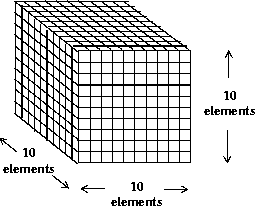
Now the 1,000 32-bit floating point numbers that were split into 1,000 SDSs are combined into one 10 x 10 x 10 element SDS. This is illustrated in the following figure.
FIGURE 14b - One 10 x 10 x 10 Element Scientific Data Set

As with the last example, 1,000 32-bit floating-point numbers are first buffered in-core, then written to the SDS. The following table contains the performance metrics of this operation.
TABLE 14B - Results of the Write Operation to One 10 x 10 x 10 Element Scientific Data Set
It is apparent from these results that merging the data into one scientific data set results in a substantial increase in I/O efficiency - in this case, a 99.9% reduction in total CPU load. In addition, the size of the HDF file is dramatically reduced by a factor of more than 100, even through the amount of SDS data stored is the same.
The extent to which the data consolidation described in this section should be done is dependent on the specific I/O requirements of the HDF user application.
14.2.2 Sharing Dimensions Between Scientific Data Sets
When several scientific data sets have dimensions of the same length, name and data type, they can share these dimensions to reduce storage overhead and CPU cycles in writing out data.
To illustrate this, again consider the example of 1,000 1 x 1 x 1 scientific data sets of 32-bit floating point numbers. Three dimensions are attached by default to each scientific data set by the HDF library. The HDF library assigns each of these dimensions a default name prefaced by "fakeDim". See Chapter 3, Scientific Data Sets (SD API), for a specific explanation of default dimension naming conventions.
FIGURE 14c - 1,000 1 x 1 x 1 Element Scientific Data Sets

One 32-bit floating point number is written to each scientific data set. The following table lists the performance metrics of this operation.
TABLE 14C - Results of the Write Operation to 1,000 1 x 1 x 1 Element Scientific Data Sets
Now consider the 1,000 SDSs described previously in this section. In this case, the 1,000 SDSs share the program-defined "X_Axis", "Y_Axis" and "Z_Axis" dimensions as illustrated in the following figure.
FIGURE 14d - 1,000 1 x 1 x 1 Element Scientific Data Sets Sharing Dimensions

The performance metrics that result from writing one 32-bit floating-point number to each dataset are in the following table.
TABLE 14D - Results of the Write Operation to 1,000 1 x 1 x 1 SDSs with Shared Dimensions
A 82% performance improvement in this example program can be seen from the information in this table, due to the fewer write operations involved in writing dimension data to shared dimensions. Also, the HDF file is significantly smaller in this case, due to the smaller amount of dimension data that is written.
14.2.3 Setting the Fill Mode
When a scientific data set is created, the default action of the HDF library is to fill every element with the default fill value. This action can be disabled, and reenabled once it has been disabled, by a call to the SDsetfillmode routine.
The library's default writing of fill values can degrade performance when, after the fill values have been written, every element in the dataset is written to again. This operation involves writing every element in the SDS twice. This section will demonstrate that disabling the initial fill value write operation by calling SDsetfillmode can improve library performance.
Consider 50 10 x 10 x 10 scientific data sets of 32-bit floating-point numbers.
FIGURE 14e - 50 10 x 10 x 10 Element Scientific Data Sets

By default, the fill value is written to every element in all 50 SDSs. The contents of a two-dimensional buffer containing 32-bit floating-point numbers is then written to these datasets. The way these two-dimensional slices are written to the three-dimensional SDSs is illustrated in the following figure. Each slice (represented by each shaded area in the figure) is written along the third dimension of each SDS, or if the dimensions are related to a Cartesian grid, the z-dimension, until the entire SDS is filled.
FIGURE 14f - Writing to the 50 10 x 10 x 10 Element Scientific Data Sets

It should be noted that the reason each SDS isn't rewritten to in one write operation is because the HDF library will detect this and automatically disable the initial write of the fill values as a performance-saving measure. Hence, the partial writes in two-dimensional slabs.
The following table shows the number of CPU cycles needed in our tests to perform this write operation with the fill value write enabled. The "Size of the HDF File" metric has been left out of this table, because it won't change substantially regardless of whether the default fill value write operation is enabled.
TABLE 14E - Results of the Write Operation to the 50 10 x 10 x 10 SDSs with the Fill Value Write Enabled
The following table shows the number of CPU cycles needed to perform the same write operation with the fill value write disabled.
TABLE 14F - Results of the Write Operation to the 50 SDSs with the Fill Value Write Disabled
The information in these tables demonstrate that eliminating the I/O overhead of the default fill value write operation when an entire SDS is rewritten to results in a substantial reduction of the CPU cycles needed to perform the operation - in this case, a reduction of 33%.
14.2.4 Disabling "Fake" Dimension Scale Values in Large One-Dimensional Scientific Data Sets
In versions 4.0 and earlier of the HDF library, dimension scales were represented by a vgroup containing a vdata. This vdata consisted of as many records as there are elements along the dimension. Each record contained one number which represented each value along the dimension scale, and these values are referred to as "fake" dimension scale values.
In HDF version 4.0 a new representation of the dimension scale was implemented alongside the old one - a vdata containing only one value representing the total number of values in the dimension scale. In version 4.1 release 1, this representation was made the default. A "compatible" mode is also supported where both the older and newer representations of the dimension scale are written to file.
In the earlier representation, a substantial amount of I/O overhead is involved in writing the fake dimension scale values into the vdata. When one of the dimensions of the SDS array is very large, performance can be improved, and the size of the HDF file can be reduced, if the old representation of dimension scales is disabled by a call to the SDsetdimval_comp routine. The examples in this section will illustrate this.
First, consider one 10,000 element array of 32-bit floating point numbers, as shown in the following figure. Both the new and old dimension scale representations are enabled by the library.
FIGURE 14g - One 10,000 Element Scientific Data Set with Old- and New-Style Dimension Scales

10,000 32-bit floating-point numbers are buffered in-core, then written to the scientific data set. In addition, 10,000 integers are written to the SDS as dimension scale values. The following table contains the results of this operation from our tests.
TABLE 14G - Results of the SDS Write Operation with the New and Old Dimension Scales
Now consider the same SDS with the fake dimension scale values disabled. The following figure illustrates this.
FIGURE 14h - One 10,000 Element Scientific Data Set With the Old-Style Dimension Scale Disabled

The following table contains the performance metrics of this write operation.
TABLE 14H - Results of the SDS Write Operation With Only the New Dimension Scale
The old-style dimension scale is not written to the HDF file, which results in the size of the file being reduced by nearly 50%. There is also a marginal reduction in the total number of CPU cycles.
[Top] [Prev] [Next]
hdfhelp@ncsa.uiuc.edu
HDF User's Guide - 07/21/98, NCSA HDF
Development Group.


