---------------------------  wave2d_45x180_example.html  --------------------------

Instructions for using this form:

1. Enter appropriate numbers in the boxes,
2. enter your email address,
3. click on submit, and
4. wait for results to be returned to your email. (this will take about 4 hours 30 minutes)
   

Simulation results returned:

1. You can either select web links in the email or view the results directly by going to the
   directory http://www.jwave.vt.edu/output/wave2d_Cij_45x180_ "unique date-time"/.
   If your email does not provide direct web links, copy and paste the web address from
   the email into your web browser location window.

2. All results are organized in one file:
   http://www.jwave.vt.edu/output/wave2d_Cij_45x180_"unique date-time" /results.html
   If the form is submitted "as-is" you can view the simulation results as an animation.

3. You should check the files wave2d_45x180.out to verify that the job ran correctly.

4. You can also download files from your web browser to your computer for archiving.
   NOTE: ALL FILES WILL BE DELETED AFTER 3 DAYS.

Below are images with back-ground-info that describes this problem in more detail.

TERMS DEFINED
==============================================================

ANIMATION: ( MPEG(768K) )

How to Visually Interpret Results
==============================================================
BULK WAVE PROPAGATION SIMULATION IN UNIDIRECTIONAL Gr/Ep
----------------------------------------------------------------------------------------------------------------
Unlike isotropic materials waves propating in anisortropic materials deviate from
the wave normal n_i. This anisotropy quides the wave energy propagation shown in
the animations provided above. From this simulation new relationships can be      
seen: 1) the faster moving QL wave has a longer wavelength, 2) diffractions         
from reflected bulk waves create Rayleigh surface waves, 3) the reflected QL       
wave energy propagates back towards the origin, 4) this refection does not             
generate another bifrucation of energy into yet another QL & QT wave. This        
information suggests that waves could be launched preferentially.                         

Because a deformed mesh shows shows the wave types, L, QL, QT, or T,
more clearly, highlighted above as red and blue regions, the animation
of simulation results are shown as a deformed mesh.

Below is specific information that describes how to use data in the form shown in the lower frame.

  __________________________________________________________________________
  Simulated transducer defined by identifying grid nodes and vibration direction angles:

========================================================================= View larger format
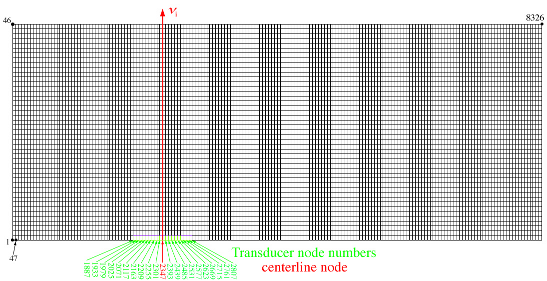
The FEM mesh size above cannot be changed in this module, however the number of nodes that define the simulated transducer (green) can be changed in the form provided in the lower frame. At the bottom of the form the user can select which nodes are active by altering the # Nodal Displ., e.g. change 21 to 11, in the first line on the form and the corresponding Number of Elements in One Wavelength which is one less that the total # Nodal Displ., e.g. change 20 to 10. The FEM program sets the Number of Elements in One Wavelength equal to the transducer length highlighted in green. For small transducers, e.g. 4 elements/wave length, the corresponding L, QL, QT, or T waves launched by the simulated transducer are equally small which gives rise to dispersion, i.e. slower wave group velocities. At 4 elements per wavelength the group velocity goes to zero. Next to the node numbers defined at the bottom of the form are the prescribed displacement directions in degrees which is set at 00.0 degrees. At 00.0 degrees these nodal displacements are restricted to move in the horizontal direction, which generates transverse waves. If these angles are set to 90.0 degrees these nodal displacements are restricted to move in the vertical direction, which generates longitidinal waves